Tuesday, April 13, 2021

New Features in Scikit learn

 Source: https://towardsdatascience.com/new-features-of-scikit-learn-fbbfe7652bfb


New Features of Scikit-Learn

Scikit-learn, Python’s machine-learning library, just got better. It’s the best time to update it.

Recently, in December 2020, scikit-learn released a major update in version 0.24. It is the last stable release of version 0. The next release will supposedly be version 1.0 and is currently in development.

I will provide an overview of some important features introduced in version 0.24. Given a large number of highlight features, I highly recommend upgrading your scikit-learn library.

Contents:

  • Upgrading to Version 0.24
  • Major Features
  • Other Interesting Features

Upgrading to Version 0.24

I am using Python environments, so, first I activated my desired environment, and then upgraded the scikit-learn version via pip.

# Activate the environment
>>> source activate py38
# Upgrade scikit-learn
>>> pip install — upgrade scikit-learn
...
...
Successfully installed scikit-learn-0.24.0

Major Features

\Photo by Tolga Ulkan on Unsplash

1) Sequential Feature Selector (SFS)

It is a way of selecting the most important features from high-dimensional spaces greedily. This transformer uses the model estimator’s cross-validation to iteratively find the best feature-subset by either adding or removing features via the forward and backward selection, respectively.

The forward selection starts with fewer features and gradually adds the best new features till the required number of features is obtained. The backward selection starts with more features and removes them one-by-one till the desired number of features is selected.

It is an alternative to the “SelectFromModel” (SFM) transformer. The advantage of SFS over SFM is that the estimator (model) used in SFS is not required to have the feature_importances_ or coef_ attribute after fitting, unlike in SFM. The disadvantage of SFS is that it is relatively slower than SFM due to its iterative nature and the k-fold CV scoring. The following is one example. Try playing around with the code using a different classifier.

from sklearn.datasets import load_wine
from sklearn.neighbors import KNeighborsClassifier
from sklearn.feature_selection import SequentialFeatureSelector
X, y = load_wine(return_X_y=True, as_frame=True)
n_features = 3
model = KNeighborsClassifier(n_neighbors=3)
sfs = SequentialFeatureSelector(model,
n_features_to_select = n_features,
direction='forward') #Try 'backward'
sfs.fit(X, y)
print("Top {} features selected by forward sequential selection:{}"\
.format(n_features, list(X.columns[sfs.get_support()])))
# Top 3 features selected by forward sequential selection:
# ['alcohol', 'flavanoids', 'color_intensity']
Photo by Markus Winkler on Unsplash

2) Individual Conditional Expectation (ICE) plots

The ICE plots are a new kind of partial dependence plots that show how a prediction for a given sample in the dataset depends on a feature. If you have 100 samples (recordings) and six features (independent variables), then you will get six subplots, where each plot will contain 100 lines (you can specify this number). The y-axes in all subplots will cover the range of the target variable (prediction), while the x-axes will cover the corresponding feature’s range.

The following code generates the ICE plots shown below.

from sklearn.datasets import load_diabetes
from sklearn.ensemble import RandomForestRegressor
X, y = load_diabetes(return_X_y=True, as_frame=True)
features = ['s1', 's2', 's3', 's4', 's5', 's6'] # features to plot
model = RandomForestRegressor(n_estimators=10)
model.fit(X, y)
ax = plot_partial_dependence(
model, X, features, kind="both", subsample=60,
line_kw={'color':'mediumseagreen'})
ax.figure_.subplots_adjust(hspace=0.4, wspace=0.1) # adjust spacing
ICE plot showing the dependence of diabetes progression onto the six blood serum features using the Random Forest Regressor.
Photo by Tamanna Rumee on Unsplash

3) Successive Halving Estimators

Two new estimators for hyperparameter tuning are introduced namely HalvingGridSearchCV and HalvingRandomSearchCV. They can respectively serve as alternatives for GridSearchCV and RandomizedSearchCV, the in-built hyperparameter tuning methods so far in scikit-learn.

The basic idea is that the search for the best hyperparameter starts on a few samples with a large set of parameters. In the next iteration, the number of samples increase (by a factor n), but the number of parameters is halved/reduced (halved does not only mean a factor of 1/2 (n=2) but can also be 1/3 (n=3), 1/4 (n=4), and so on). This halving procedure continues till the final iteration. Finally, the best subset of parameters is the one that has the highest score in the last iteration.

Similar to the existing two methods, the “successive halving” can either be performed randomly (HavingRandomSearchCV) or exhaustively (HavingGridSearchCV). The following example demonstrates the use case of HavingRandomSearchCV (you can similarly use HavingGridSearchCV). For a comprehensive explanation of how to choose the best parameters, refer here.

from sklearn.datasets import load_iris
from sklearn.ensemble import RandomForestClassifier
from sklearn.model_selection import HalvingRandomSearchCV
X, y = load_iris(return_X_y=True, as_frame=True)
model = RandomForestClassifier(random_state=123, n_jobs=-1)
param_grid = {"n_estimators": [20, 50, 100],
"bootstrap": [True, False],
"criterion": ["gini", "entropy"],
"max_depth": [1, 2, 3],
"max_features": randint(1, 5),
"min_samples_split": randint(2, 9)
}
grid = HalvingRandomSearchCV(estimator=model,
param_distributions=param_grid,
factor=2, random_state=123,)
grid.fit(X, y)
print(grid.best_params_)
# Output
{'bootstrap': True, 'criterion': 'gini', 'max_depth': 2, 'max_features': 4, 'min_samples_split': 8, 'n_estimators': 50}
Photo by Rhodi Lopez on Unsplash

4) Semi-supervised Self Training Classifier

Scikit-learn has several classifiers for supervised learning. Now it is possible for these supervised classifiers to perform a semi-supervised classification, i.e. enabling the model to learn from unlabeled data. Only those classifiers that predict class probabilities for the target variable can be used as semi-supervised classifiersThe official example here provides a comparison of supervised and semi-supervised classification for the Iris dataset.

The following articles nicely explain the concept of semi-supervised learning:

Photo by Anastasia Zhenina on Unsplash

5) Native categorical features in HistGradientBoosting

Both, the ‘HistGradientBoostingRegressor’ and the ‘HistGradientBoostingClassifier’ now can support categorical features that are non-ordered. Generally, one has to encode the categorical features using schemes such as One-Hot Encoding, Ordinal Labeling, etc. With the new native feature, one can directly specify the categorical columns (features) without needing to encode them.

The best part is that the missing values can be treated as a separate category. Typically, the One-Hot Encoding is applied to the training set. For a given feature (column), suppose the training set has six categories, and the test set has seven. In such a situation, the model trained on six additional columns (one extra feature per category value due to the One-Hot Encoding transformation) will throw an error during the validation on the test set due to the unknown 7th category. The native feature can circumvent this problem by considering this 7th unknown category as missing values.

Refer to this official example comparing different encoding schemes.

6) What NOT to do with scikit-learn

New documentation is added that focuses on the common pitfalls while machine learning using scikit-learn. Along with highlighting the common mistakes, it also explains the recommended ways to do certain things. Some examples covered in this documentation includes:

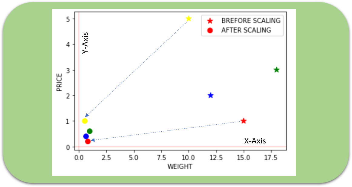
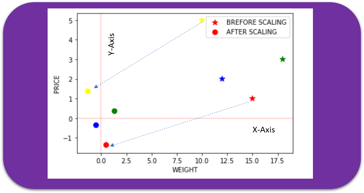
  • Best practices for data transformation (e.g., standardization)
  • The correct interpretation of the coefficients of linear models
  • Avoiding data leakage by correct handling of train and test datasets
  • Recommended use of the random state to control the randomness, e.g., during the k-fold CV

Additional Documentation

Typically, GridSearchCV is used to find the best subset of hyperparameters for our model. Based on our predefined performance scoring parameter (e.g., 'accuracy' or 'recall' or 'precision' etc.), we choose the best hyperparameter subset. This documentation provides an example demonstrating the correct way to compare different models in terms of their statistical significance.

Other Interesting Features

1) New evaluation metric for regression

Mean absolute percentage error (MAPE) is a new evaluation metric introduced for regression problems. This metric is insensitive to the global scaling of the target variable. It is a fair measure of the error in situations where the data ranges over several orders of magnitude by computing the relative percentage of error w.r.t true values. Refer to this page for more details.

Mean Absolute Percentage Error. ϵ is an arbitrarily small positive number, for example, 1e-6. The variables y and y_hat represent true and predicted values.

2) One-Hot Encoder treats missing values as categories

The One-Hot Encoder can now treat the missing values in a categorical feature as an additional category. If the missing values in a particular categorical-feature are 'None' and 'np.nan', they will be encoded as two separate categories.

3) Encoding unknown categories using OrdinalEncoder

The OrdinalEncoder now allows encoding the unknown categories during transformation to a user-specified value.

4) Poisson splitting criterion for DecisionTreeRegressor

DecisionTreeRegressor now supports a new splitting criterion called 'poisson' that splits a node based on a reduction in Poisson’s deviance. It is helpful to model situations in which the target variable represents a count or a frequency. Refer to this article for more on Poisson distribution.

5) Optional color bar in confusion matrix plot

The color bar is now optional while plotting the confusion matrix. To achieve this, you have to pass the keyword colorbar=False.

plot_confusion_matrix(estimator, X, y, colorbar=False)

Conclusion

This post lists some of the highlight changes in the latest scikit-learn update (v0.24). The complete list of changes is available here. It was the last update for version 0. The next version will be 1.0. If you are interested in knowing the highlight features in the previous version (v0.23), check out my earlier post:

Saturday, December 12, 2020

All about Feature Scaling


IN DEPTH ANALYSIS

All about Feature Scaling

Scale data for better performance of Machine Learning Model

Machine learning is like making a mixed fruit juice. If we want to get the best-mixed juice, we need to mix all fruit not by their size but based on their right proportion. We just need to remember apple and strawberry are not the same unless we make them similar in some context to compare their attribute. Similarly, in many machine learning algorithms, to bring all features in the same standing, we need to do scaling so that one significant number doesn’t impact the model just because of their large magnitude.

Feature scaling in machine learning is one of the most critical steps during the pre-processing of data before creating a machine learning model. Scaling can make a difference between a weak machine learning model and a better one.

The most common techniques of feature scaling are Normalization and Standardization.

Normalization is used when we want to bound our values between two numbers, typically, between [0,1] or [-1,1]. While Standardization transforms the data to have zero mean and a variance of 1, they make our data unitless. Refer to the below diagram, which shows how data looks after scaling in the X-Y plane.

Image for post

Why do we need scaling?

Machine learning algorithm just sees number — if there is a vast difference in the range say few ranging in thousands and few ranging in the tens, and it makes the underlying assumption that higher ranging numbers have superiority of some sort. So these more significant number starts playing a more decisive role while training the model.

The machine learning algorithm works on numbers and does not know what that number represents. A weight of 10 grams and a price of 10 dollars represents completely two different things — which is a no brainer for humans, but for a model as a feature, it treats both as same.

Suppose we have two features of weight and price, as in the below table. The “Weight” cannot have a meaningful comparison with the “Price.” So the assumption algorithm makes that since “Weight” > “Price,” thus “Weight,” is more important than “Price.”

Image for post

So these more significant number starts playing a more decisive role while training the model. Thus feature scaling is needed to bring every feature in the same footing without any upfront importance. Interestingly, if we convert the weight to “Kg,” then “Price” becomes dominant.

Another reason why feature scaling is applied is that few algorithms like Neural network gradient descent converge much faster with feature scaling than without it.

Image for post
Photo Credit

One more reason is saturation, like in the case of sigmoid activation in Neural Network, scaling would help not to saturate too fast.

When to do scaling?

Feature scaling is essential for machine learning algorithms that calculate distances between data. If not scale, the feature with a higher value range starts dominating when calculating distances, as explained intuitively in the “why?” section.

The ML algorithm is sensitive to the “relative scales of features,” which usually happens when it uses the numeric values of the features rather than say their rank.

In many algorithms, when we desire faster convergence, scaling is a MUST like in Neural Network.

Since the range of values of raw data varies widely, in some machine learning algorithms, objective functions do not work correctly without normalization. For example, the majority of classifiers calculate the distance between two points by the distance. If one of the features has a broad range of values, the distance governs this particular feature. Therefore, the range of all features should be normalized so that each feature contributes approximately proportionately to the final distance.

Even when the conditions, as mentioned above, are not satisfied, you may still need to rescale your features if the ML algorithm expects some scale or a saturation phenomenon can happen. Again, a neural network with saturating activation functions (e.g., sigmoid) is a good example.

Rule of thumb we may follow here is an algorithm that computes distance or assumes normality, scales your features.

Some examples of algorithms where feature scaling matters are:

  • K-nearest neighbors (KNN) with a Euclidean distance measure is sensitive to magnitudes and hence should be scaled for all features to weigh in equally.
  • K-Means uses the Euclidean distance measure here feature scaling matters.
  • Scaling is critical while performing Principal Component Analysis(PCA). PCA tries to get the features with maximum variance, and the variance is high for high magnitude features and skews the PCA towards high magnitude features.
  • We can speed up gradient descent by scaling because θ descends quickly on small ranges and slowly on large ranges, and oscillates inefficiently down to the optimum when the variables are very uneven.

Algorithms that do not require normalization/scaling are the ones that rely on rules. They would not be affected by any monotonic transformations of the variables. Scaling is a monotonic transformation. Examples of algorithms in this category are all the tree-based algorithms — CART, Random Forests, Gradient Boosted Decision Trees. These algorithms utilize rules (series of inequalities) and do not require normalization.

Algorithms like Linear Discriminant Analysis(LDA), Naive Bayes is by design equipped to handle this and give weights to the features accordingly. Performing features scaling in these algorithms may not have much effect.

Few key points to note :

  • Mean centering does not affect the covariance matrix
  • Scaling of variables does affect the covariance matrix
  • Standardizing affects the covariance

How to perform feature scaling?

Below are the few ways we can do feature scaling.

1) Min Max Scaler
2) Standard Scaler
3) Max Abs Scaler
4) Robust Scaler
5) Quantile Transformer Scaler
6) Power Transformer Scaler
7) Unit Vector Scaler

For the explanation, we will use the table shown in the top and form the data frame to show different scaling methods.

import pandas as pd
import numpy as np
import matplotlib.pyplot as plt
%matplotlib inline
df = pd.DataFrame({'WEIGHT': [15, 18, 12,10],
'PRICE': [1,3,2,5]},
index = ['Orange','Apple','Banana','Grape'])
print(df)
WEIGHT PRICE
Orange 15 1
Apple 18 3
Banana 12 2
Grape 10 5

1)Min-Max scaler

Image for post

Transform features by scaling each feature to a given range. This estimator scales and translates each feature individually such that it is in the given range on the training set, e.g., between zero and one. This Scaler shrinks the data within the range of -1 to 1 if there are negative values. We can set the range like [0,1] or [0,5] or [-1,1].

This Scaler responds well if the standard deviation is small and when a distribution is not Gaussian. This Scaler is sensitive to outliers.

from sklearn.preprocessing import MinMaxScaler
scaler = MinMaxScaler()
df1 = pd.DataFrame(scaler.fit_transform(df),
columns=['WEIGHT','PRICE'],
index = ['Orange','Apple','Banana','Grape'])ax = df.plot.scatter(x='WEIGHT', y='PRICE',color=['red','green','blue','yellow'],
marker = '*',s=80, label='BREFORE SCALING');
df1.plot.scatter(x='WEIGHT', y='PRICE', color=['red','green','blue','yellow'],
marker = 'o',s=60,label='AFTER SCALING', ax = ax);
plt.axhline(0, color='red',alpha=0.2)
plt.axvline(0, color='red',alpha=0.2);
Image for post

2) Standard Scaler

Image for post

The Standard Scaler assumes data is normally distributed within each feature and scales them such that the distribution centered around 0, with a standard deviation of 1.

Centering and scaling happen independently on each feature by computing the relevant statistics on the samples in the training set. If data is not normally distributed, this is not the best Scaler to use.

from sklearn.preprocessing import StandardScaler
scaler = StandardScaler()
df2 = pd.DataFrame(scaler.fit_transform(df),
columns=['WEIGHT','PRICE'],
index = ['Orange','Apple','Banana','Grape'])
ax = df.plot.scatter(x='WEIGHT', y='PRICE',color=['red','green','blue','yellow'],
marker = '*',s=80, label='BREFORE SCALING');
df2.plot.scatter(x='WEIGHT', y='PRICE', color=['red','green','blue','yellow'],
marker = 'o',s=60,label='AFTER SCALING', ax = ax)
plt.axhline(0, color='red',alpha=0.2)
plt.axvline(0, color='red',alpha=0.2);
Image for post

3) Max Abs Scaler

Scale each feature by its maximum absolute value. This estimator scales and translates each feature individually such that the maximal absolute value of each feature in the training set is 1.0. It does not shift/center the data and thus does not destroy any sparsity.

On positive-only data, this Scaler behaves similarly to Min Max Scaler and, therefore, also suffers from the presence of significant outliers.

from sklearn.preprocessing import MaxAbsScaler
scaler = MaxAbsScaler()
df4 = pd.DataFrame(scaler.fit_transform(df),
columns=['WEIGHT','PRICE'],
index = ['Orange','Apple','Banana','Grape'])
ax = df.plot.scatter(x='WEIGHT', y='PRICE',color=['red','green','blue','yellow'],
marker = '*',s=80, label='BREFORE SCALING');
df4.plot.scatter(x='WEIGHT', y='PRICE', color=['red','green','blue','yellow'],
marker = 'o',s=60,label='AFTER SCALING', ax = ax)
plt.axhline(0, color='red',alpha=0.2)
plt.axvline(0, color='red',alpha=0.2);
Image for post

4) Robust Scaler

As the name suggests, this Scaler is robust to outliers. If our data contains many outliers, scaling using the mean and standard deviation of the data won’t work well.

This Scaler removes the median and scales the data according to the quantile range (defaults to IQR: Interquartile Range). The IQR is the range between the 1st quartile (25th quantile) and the 3rd quartile (75th quantile). The centering and scaling statistics of this Scaler are based on percentiles and are therefore not influenced by a few numbers of huge marginal outliers. Note that the outliers themselves are still present in the transformed data. If a separate outlier clipping is desirable, a non-linear transformation is required.

from sklearn.preprocessing import RobustScaler
scaler = RobustScaler()
df3 = pd.DataFrame(scaler.fit_transform(df),
columns=['WEIGHT','PRICE'],
index = ['Orange','Apple','Banana','Grape'])
ax = df.plot.scatter(x='WEIGHT', y='PRICE',color=['red','green','blue','yellow'],
marker = '*',s=80, label='BREFORE SCALING');
df3.plot.scatter(x='WEIGHT', y='PRICE', color=['red','green','blue','yellow'],
marker = 'o',s=60,label='AFTER SCALING', ax = ax)
plt.axhline(0, color='red',alpha=0.2)
plt.axvline(0, color='red',alpha=0.2);
Image for post

Let’s now see what happens if we introduce an outlier and see the effect of scaling using Standard Scaler and Robust Scaler (a circle shows outlier).

dfr = pd.DataFrame({'WEIGHT': [15, 18, 12,10,50],
'PRICE': [1,3,2,5,20]},
index = ['Orange','Apple','Banana','Grape','Jackfruit'])
print(dfr)
from sklearn.preprocessing import StandardScaler
scaler = StandardScaler()
df21 = pd.DataFrame(scaler.fit_transform(dfr),
columns=['WEIGHT','PRICE'],
index = ['Orange','Apple','Banana','Grape','Jackfruit'])
ax = dfr.plot.scatter(x='WEIGHT', y='PRICE',color=['red','green','blue','yellow','black'],
marker = '*',s=80, label='BREFORE SCALING');
df21.plot.scatter(x='WEIGHT', y='PRICE', color=['red','green','blue','yellow','black'],
marker = 'o',s=60,label='STANDARD', ax = ax,figsize=(12,6))
from sklearn.preprocessing import RobustScaler
scaler = RobustScaler()
df31 = pd.DataFrame(scaler.fit_transform(dfr),
columns=['WEIGHT','PRICE'],
index = ['Orange','Apple','Banana','Grape','Jackfruit'])
df31.plot.scatter(x='WEIGHT', y='PRICE', color=['red','green','blue','yellow','black'],
marker = 'v',s=60,label='ROBUST', ax = ax,figsize=(12,6))
plt.axhline(0, color='red',alpha=0.2)
plt.axvline(0, color='red',alpha=0.2);
WEIGHT PRICE
Orange 15 1
Apple 18 3
Banana 12 2
Grape 10 5
Jackfruit 50 20
Image for post

5) Quantile Transformer Scaler

Transform features using quantiles information.

This method transforms the features to follow a uniform or a normal distribution. Therefore, for a given feature, this transformation tends to spread out the most frequent values. It also reduces the impact of (marginal) outliers: this is, therefore, a robust pre-processing scheme.

The cumulative distribution function of a feature is used to project the original values. Note that this transform is non-linear and may distort linear correlations between variables measured at the same scale but renders variables measured at different scales more directly comparable. This is also sometimes called as Rank scaler.

from sklearn.preprocessing import QuantileTransformer
scaler = QuantileTransformer()
df6 = pd.DataFrame(scaler.fit_transform(df),
columns=['WEIGHT','PRICE'],
index = ['Orange','Apple','Banana','Grape'])
ax = df.plot.scatter(x='WEIGHT', y='PRICE',color=['red','green','blue','yellow'],
marker = '*',s=80, label='BREFORE SCALING');
df6.plot.scatter(x='WEIGHT', y='PRICE', color=['red','green','blue','yellow'],
marker = 'o',s=60,label='AFTER SCALING', ax = ax,figsize=(6,4))
plt.axhline(0, color='red',alpha=0.2)
plt.axvline(0, color='red',alpha=0.2);
Image for post

The above example is just for illustration as Quantile transformer is useful when we have a large dataset with many data points usually more than 1000.

6) Power Transformer Scaler

The power transformer is a family of parametric, monotonic transformations that are applied to make data more Gaussian-like. This is useful for modeling issues related to the variability of a variable that is unequal across the range (heteroscedasticity) or situations where normality is desired.

The power transform finds the optimal scaling factor in stabilizing variance and minimizing skewness through maximum likelihood estimation. Currently, Sklearn implementation of PowerTransformer supports the Box-Cox transform and the Yeo-Johnson transform. The optimal parameter for stabilizing variance and minimizing skewness is estimated through maximum likelihood. Box-Cox requires input data to be strictly positive, while Yeo-Johnson supports both positive or negative data.

from sklearn.preprocessing import PowerTransformer
scaler = PowerTransformer(method='yeo-johnson')
df5 = pd.DataFrame(scaler.fit_transform(df),
columns=['WEIGHT','PRICE'],
index = ['Orange','Apple','Banana','Grape'])
ax = df.plot.scatter(x='WEIGHT', y='PRICE',color=['red','green','blue','yellow'],
marker = '*',s=80, label='BREFORE SCALING');
df5.plot.scatter(x='WEIGHT', y='PRICE', color=['red','green','blue','yellow'],
marker = 'o',s=60,label='AFTER SCALING', ax = ax)
plt.axhline(0, color='red',alpha=0.2)
plt.axvline(0, color='red',alpha=0.2);
Image for post

7) Unit Vector Scaler

Image for post

Scaling is done considering the whole feature vector to be of unit length. This usually means dividing each component by the Euclidean length of the vector (L2 Norm). In some applications (e.g., histogram features), it can be more practical to use the L1 norm of the feature vector.

Like Min-Max Scaling, the Unit Vector technique produces values of range [0,1]. When dealing with features with hard boundaries, this is quite useful. For example, when dealing with image data, the colors can range from only 0 to 255.

Image for post

If we plot, then it would look as below for L1 and L2 norm, respectively.

Image for post

The below diagram shows how data spread for all different scaling techniques, and as we can see, a few points are overlapping, thus not visible separately.

Image for post

Final Note:

Feature scaling is an essential step in Machine Learning pre-processing. Deep learning requires feature scaling for faster convergence, and thus it is vital to decide which feature scaling to use. There are many comparison surveys of scaling methods for various algorithms. Still, like most other machine learning steps, feature scaling too is a trial and error process, not a single silver bullet.

I look forward to your comment and share if you have any unique experience related to feature scaling. Thanks for reading. You can connect me @LinkedIn.

Reference:

http://sebastianraschka.com/Articles/2014_about_feature_scaling.html

https://www.kdnuggets.com/2019/04/normalization-vs-standardization-quantitative-analysis.html

https://scikit-learn.org/stable/modules/preprocessing.html

WRITTEN BY

Data Science | Machine Learning | Deep Learning | Artificial Intelligence