Custom Machine Learning Pipeline in production

Custom ML Pipeline is built using OOP programming.

In OOP, we write code in the form of objects.
The objects can store data  and can also store instructions or procedures to modify that data.
       Data => attributes.
       Instructions pr procedures => methods.

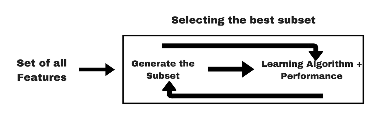
A pipeline is a set of data processing steps connected in series, where typically, the output of one element is the input of the next one.

The element of a pipeline can be executed in parallel or in time-sliced fashion. This is useful when we require use of big data or high computing power eg: neural networks.

So, a custom ml pipeline is a sequence of steps, aimed at loading and transforming data, to get it ready for training or scoring where:
   - We write processing steps as objects(OOP)
   - We write sequence i.e pipeline as objects (OOP)

Refer: customPipelineProcessor.py
           customPipelineTrain.py




Leveraging Third party pipeline : Scikit-Learn




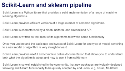
How is scikit-learn organized?




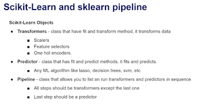
The characteristics of scikit-learn pipeline is such that, you can have as many transformers as you want and all of them except the last one, the last one should be a predictor.




Feature creation and Feature engineering steps as Scikit-learn Objects.

Transformers: class that have fit an transform method, it transforms data.
Use of scikit-learn base transformers
     Inherit class and adjust the fit and transform methods.

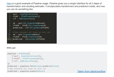
Scikit-Learn Pipeline - Code

Below the code for the Scikit-Learn pipeline, utilising the transformers we created in the previous lecture. Briefly, we list inside the pipeline, the different transformers, in the order they should run. The final step is the linear model. Right in front of the linear model, we should run the Scaler.

You will better understand the structure of the code in the coming lectures. Briefly, we write the transformers in a script within a folder called processing. We also write a config file, where we specify the categorical and numerical variables. Bear with us and we will show you all the scripts. For now, make sure you understand well how to write a scikit-learn pipeline.

from sklearn.linear_model import Lasso
from sklearn.pipeline import Pipeline
from sklearn.preprocessing import MinMaxScaler
 
from regression_model.config import config
from regression_model.processing import preprocessors as pp
 
price_pipe = Pipeline([
                ('categorical_imputer', pp.CategoricalImputer(variables = config.CATEGORICAL_VARS_WITH_NA)),
                ('numerical_inputer', pp.NumericalImputer(variables = config.NUMERICAL_VARS_WITH_NA)),
                ('temporal_variable', pp.TemporalVariableEstimator(variables=config.TEMPORAL_VARS, reference_variable=config.REFERENCE_TEMP_VAR)),
                ('rare_label_encoder', pp.RareLabelCategoricalEncoder(tol = 0.01, variables = config.CATEGORICAL_VARS)),
                ('categorical_encoder', pp.CategoricalEncoder(variables=config.CATEGORICAL_VARS)),
                ('log_transformer', pp.LogTransformer(variables = config.NUMERICALS_LOG_VARS)),
                ('drop_features', pp.DropUnecessaryFeatures(variables_to_drop = config.DROP_FEATURES)),
                ('scaler', MinMaxScaler()),
                ('Linear_model', Lasso(alpha=0.005, random_state=0))
            ])

Should feature selection be part of the pipeline?

Scikit-Learn and sklearn pipeline: Additional reading resources


Introduction to Scikit-Learn
Six reasons why I recommend Scikit-Learn
Why you should learn Scikit-Learn
Deep dive into SKlearn pipelines from Kaggle
SKlearn pipeline tutorial from Kaggle
Managing Machine Learning workflows with Sklearn pipelines
A simple example of pipeline in Machine Learning using SKlearn







Resources to Improve as a Python Developer


Become a better python developer

We have gathered the following resources for data scientists who want to learn best practices in python programming.


The Best of the Best Practices (BOBP) Guide for Python
Python coding standards/best practices in Stackoverflow
Python Best Practices for More Pythonic Code
The Hitchhickers guide to python
Tutorials for pycharm here and here.

Writing Production code for Machine learning deployment

Overview

Most likely, you would have your ML pipeline code for the research environment in tools like Jupyter Notebook.

So we need to code in production for:
  Create and transform features.
  Incorporate the feature selection.
  Build ml models.
  Score new data.




There are three main ways for writing ML pipeline in production.

 Procedural Programming - Sequence of functions like Jupyter notebooks.
 Custom pipeline code - OOPS way that calls the procedures in order.
 Third party pipeline code - OOPS way that calls the procedures in order of third party. eg; scikit learn

Procedural Programming

 In Procedural Programming, procedures, also known as routines, subroutines or functions, are carried out as a series of computational steps.

Here is refers to writing the series of feature creation, feature transformation, model training and data scoring steps as functions, that we can call and run one after the other.


We keep following things in the yaml file

Hard coded variables to engineer, and values to use to transform features.

Hardcoded paths to retrieve and store data

By changing these values, we can re-adjust out models.

Building a Reproducible Machine learning Pipeline

Problems that we normally encounter when we build machine learning pipelines and how we make sure we minimize them by implementing the correct design of ml pipeline right from the start.

Lack of reproducibility can have significant financial cost. Also lost of time and potential loss of reputation.



Remember we just don't deploy ml models, we deploy entire ml pipeline, so we need to make sure every step of pipeline is reproducible. In the ML pipeline(refer Machine Learning Model Pipeline Overview), All the steps except Data analysis need reproducibility. So all these steps must produce identical result given the same data both in research and deployed production env.



In case of SQL loading(random loading), if the data that was loaded in one env does not coincide with another env, we will have reproducibility problems. This comes from the fact that, when we divide the train and test set, we utilize the random function, so we need the training set in another env(research and production) is exactly the same. We solve this via keeping the same seed in the random function between envs.

Also when we store snapshot of data, with GDPR, you might not be allowed to store data other than the source.







Neural networks pose particular challenge because we need to set the seed on several occasions, depending on the pattern we are using to try and make reusable many random initializations parameters it need in order to be trained. So In NN, all the required seeds needs to be saved.





Much of the loss of benefit that the model should provide comes from incomplete or erroneous integration of the models with the other systems environment.

Additional Resources.

Building a Reproducible Machine Learning Pipeline

Introducing FBLearner Flow: Facebook’s AI backbone

Scaling Machine Learning as a service: Uber’s pipeline

A systems perspective to reproducibility in Production Machine Learning

Hidden technical debt in machine learning systems

REST API Machine Learning Architecture

Architecture Component breakdown (ML Application)

Train by batch, predict on the fly.



Breakdown: Training Phase (done offline/ train by batch)






Training data:  applications will be responsible for loading, processing and giving access to the training data(could be pulling data from multiple SQL or NoSQL databases, HDFS, or make API calls), perform pre processing steps to get to the format required by scikit-learn, tensorflow or another ml framework.

Feature Extractor
There will be Applications and scripts to create features, extract features(can be simple scripts or entire models itself)

Model Builder
This includes serializing and persisting models, versioning them, making sure they are in the format suitable for deployment. In python context, this would involve in packaging with a set of py files.
In Java or Scala, we might export to an mlib bundle/jar files.

All three steps will be structured into a pipeline perhaps with scikit learn or when performance is important then Apache Spark. These piplelines will be run by CI/CD platforms to automate the work.

The output is a trained model, which can be easily deployed via REST API.

Breakdown: Prediction Phase

The model is now deployed to production to give results in real time. Requests are sent to our REST API, cleaned and prepared by the preprocessing and feature extraction code. We should mirror the code used in training as close as possible.
Prediction are given by our loaded model.

Our API can do both single and bulk predictions, where bulk predictions are subject to performance tuning and throttling.




Everything when put together, we can offline and online part of the system.





It is important to see where the code overlaps. For eg: Feature extractor(extracting features of the input given by clients to REST API as same features decided on the train time) code.

There are other components required to make the entire system running apart from application.

Entire System Diagram





Top left is the application part with examples of tools and frameworks. CI/CD pipeline sits in the middle. Our application code can be converted into docker images and stored in image registery such as docker hub or AWS Elastic container registry for easy to track and deploy. We can persist our trained model to file servers such as Gemfury or Amazon S3. Code sits in Github to manage effectively, to version, collaborate and host the code. All these steps with CI/CD pipeline. Finally we deploy the applications to either managed cloud platforms like Heroku or our own configured cloud infrastructure such as AWS Elastic container service. With this systems in place we can server our predictions via REST API as requests come in from clients.

Clarity on architecture and trade offs are important before embarking into complex development project, particularly with ml systems.

Design Approaches to ML System Architecture

General ML Architectures

1. Train by batch, predict on the fly, serve via REST API.
     The model trained and persisted offline, loaded into a web application, and give real time predictions of the input data given by client via REST API.
2. Train by batch, predict by batch, server through a shared database.

3. Train, predict by streaming.

4. Train by batch, predict on mobile(or other client).

In Pattern1 we are able to serve predictions almost in real time, so it means its easy to A/B test as well.
One of the problem here is, since we are doing this on the fly, we are not able use a slow algorithm, and there is a complexity in scaling.

In Pattern2, It is easy to use a different systems for front end and different system for batch, so different languages, different frameworks can be used. Easier to manage model version and prediction results. We can use an slow and complex algorithm. On the other side, there is lag between prediction to ingesting, so not suitable for many types of consumer applications.

In Pattern3, We can predict with very low latency and we can update the model interactively. On the con side this requires some complex infrastructure.

In Pattern4, We would have low latency for prediction, but we have tight coupling with the device, so we are limited to number of algorithms that are available to use on the device.

Patten1 is the best trade off for most cases.

Machine Learning System Architecture

What is Architecture?

In simple terms, the way software components are arranged and the interactions between them.

Why is it important at the start?

Maintaining ML systems is challenging. They have all the tech debts issues of traditional systems +
issues of its own.

So, Clarity in planning and architecture design helps to mitigate potential issues and errors.

A shared understanding of the system architecture and responsibilities is essential for effective cooperation between data science, engineering, and devops teams.

Specific Challenges of ml systems

1. The need for reproducibility(versioning everywhere)
   This is essentially the ability to duplicate the ml model exactly, this can be necessary for research, model improvements, audits or regulatory reasons depending on the business.

2. Entanglement
   If we have an input feature that we change then the importance, weights or use of the remaining features may all change as well. So there is a challenge of input not being independent, this is refers as change in anything changes everything principle.

3. Data dependencies

4. Configuration issues.
 There is a need for incrementing models and experimenting, this can result in temptation to build models on top of each other and create subtle dependencies. There is a challenge of allowing configurations to be flexible, making it easy to see difference in configuration between two models. This is not straight forward and requires specific steps to be taken.

5. Data and feature preparation.
  Systems can run the risk of massive amount of supporting code written to get data into and out to expected formats. eg: for scikit learn or tensorflow consumption.

6. Model errors can he hard to detect with traditional tests.
 
7. Separation of Expertise



So we have Data Scientists developing the model. Software engineers taking the models and putting them into applications, devops doing the deployments and business having executives, product managers determining what their requirements are. In this context there is a risk of code being thrown over the wall from departments to another, when no one understands the full process. So mitigating the risk of errors and wasted time is important.

Best resources for machine learning

https://www.trainindata.com/post/best-resources-to-learn-machine-learning

Model Building

http://localhost:8888/notebooks/Desktop/TechStack/DMLM/MLPipeline-Notebooks/02.9_ML_Pipeline_Step4-MachineLearningModelBuild.ipynb

Feature Engineering

http://localhost:8888/notebooks/Desktop/TechStack/DMLM/MLPipeline-Notebooks/02.7_ML_Pipeline_Step2-FeatureEngineering.ipynb

Why seeding is important during research and development/production env for ml model?

It is important to note that we are engineering variables and pre-processing data with the idea of deploying the model if we find business value in it. Therefore, from now on, for each step that includes some element of randomness, it is extremely important that we set the seed. This way, we can obtain reproducibility between our research and our development code. Reproducibility here means same output comes for same input during reaseach and development(production deployment) code.

Why do we want to set the seed? Manny of the ml algorithm we use, involves element of randomness. Settting the seed makes the reproducibility between research and production/development env possible and control the randomness.

This is perhaps one of the most important lessons that you need to take away from this course: Always set the seeds.

What is seeding?

>>> import random
>>> random.seed(9001)
>>> random.randint(1, 10)
1
>>> random.randint(1, 10)
3
>>> random.randint(1, 10)
6
>>> random.randint(1, 10)
6
>>> random.randint(1, 10)
7

Pseudo-random number generators work by performing some operation on a value. Generally this value is the previous number generated by the generator. However, the first time you use the generator, there is no previous value.

Seeding a pseudo-random number generator gives it its first "previous" value. Each seed value will correspond to a sequence of generated values for a given random number generator. That is, if you provide the same seed twice, you get the same sequence of numbers twice.

Generally, you want to seed your random number generator with some value that will change each execution of the program. For instance, the current time is a frequently-used seed. The reason why this doesn't happen automatically is so that if you want, you can provide a specific seed to get a known sequence of numbers.

Why do we need randomness?
https://www.kdnuggets.com/2017/06/surprising-complexity-randomness.html


Embrace randomness in machine learning

https://machinelearningmastery.com/randomness-in-machine-learning/

Reproducible machine learning
http://www.rctatman.com/files/Tatman_2018_ReproducibleML.pdf

Machine learning reproducibility crisis.
https://petewarden.com/2018/03/19/the-machine-learning-reproducibility-crisis/

Regularization

Pre-step:
Bias and Variance:

https://www.youtube.com/watch?v=EuBBz3bI-aA&list=PLblh5JKOoLUICTaGLRoHQDuF_7q2GfuJF&index=5

 1. Ridge Regularization

https://www.youtube.com/watch?v=Q81RR3yKn30
    
2. Lasso Regularization

https://www.youtube.com/watch?v=NGf0voTMlcs


3. Elastic net Regularization. 

https://www.youtube.com/watch?v=1dKRdX9bfIo

Data analysis

http://localhost:8888/notebooks/Desktop/TechStack/DMLM/MLPipeline-Notebooks/02.6_ML_Pipeline_Step1-DataAnalysis.ipynb

Machine learning Model Pipeline: Model building

We can build various models like linear models. for eg: linear regression models(MARS). We can build decision tree based models like random forest, gradient boosted trees. We can also build neural networks. We can also build clustering algorithms.
And then when we pass the pre processed data to the model, we get the prediction that they make.



We need to then evaluate the performance of
predictions that this model make.

For classification we can measure the ROC-AUC which gives us the indication that how many times the model makes good assessment
vs how many times the model makes wrong assessment.





Some time we also build multiple ml algorithms and then build the meta model that takes in prediction  of all the initial models and combines them to make better assessment of the target. This is called Meta Ensembling.



We can have this also as a pipeline of Meta ensembling for model deployment.

Machine learning model Pipeline: Feature Selection

 Feature selection refers to a phase in which we use algorithms or procedures to choose best subset of features from all the variables/feature present in your dataset. This is the process of finding the most predictive features for the model we are trying to build.

At the beginning of feature selection process, we start with entire dataset with all the variables and by the end we end up with small set of variables that are most predictive ones.

Why do we select features ?

Simple models are easier to interpret.

Shorter training times and more importantly lesser time to score when we use less features.

Enhanced generalisation by reducing overfitting.

Easier to implement by Software engineers -> model in production.

Reduced risk of data errors during model use.

Data redundancy i.e many features provide the same information.

Why having less features is important for model deployment to production?

 Smaller json messages sent over to the model.
   Json messages contain only the necessary variables / inputs

Less lines of code for error handling
  Error handlers need to be written for each variable/ input.
  Typically we write error handlers for each and every variable we send to model.

Less information to log.

Less feature engineering code.

Variable Redundancy



Feature Selection Methods


 

Filter methods

Filter methods are generally used as a preprocessing step. The selection of features is independent of any machine learning algorithms. Instead, features are selected on the basis of their scores in various statistical tests for their correlation with the outcome variable. The correlation is a subjective term here. For basic guidance, you can refer to the following table for defining correlation co-efficients.

• Pearson’s Correlation: It is used as a measure for quantifying linear dependence between two continuous variables X and Y. Its value varies from -1 to +1. Pearson’s correlation is given as:

• LDA: Linear discriminant analysis is used to find a linear combination of features that characterizes or separates two or more classes (or levels) of a categorical variable.

• ANOVA: ANOVA stands for Analysis of variance. It is similar to LDA except for the fact that it is operated using one or more categorical independent features and one continuous dependent feature. It provides a statistical test of whether the means of several groups are equal or not.

• Chi-Square: It is a is a statistical test applied to the groups of categorical features to evaluate the likelihood of correlation or association between them using their frequency distribution.

One thing that should be kept in mind is that filter methods do not remove multicollinearity. So, you must deal with multicollinearity of features as well before training models for your data.

Wrapper methods

In wrapper methods, we try to use a subset of features and train a model using them. Based on the inferences that we draw from the previous model, we decide to add or remove features from your subset. The problem is essentially reduced to a search problem. These methods are usually computationally very expensive.

Some common examples of wrapper methods are forward feature selection, backward feature elimination, recursive feature elimination, etc.

• Forward Selection: Forward selection is an iterative method in which we start with having no feature in the model. In each iteration, we keep adding the feature which best improves our model till an addition of a new variable does not improve the performance of the model.
• Backward Elimination: In backward elimination, we start with all the features and removes the least significant feature at each iteration which improves the performance of the model. We repeat this until no improvement is observed on removal of features.
• Recursive Feature elimination: It is a greedy optimization algorithm which aims to find the best performing feature subset. It repeatedly creates models and keeps aside the best or the worst performing feature at each iteration. It constructs the next model with the left features until all the features are exhausted. It then ranks the features based on the order of their elimination.

One of the best ways for implementing feature selection with wrapper methods is to use Boruta package that finds the importance of a feature by creating shadow features.

It works in the following steps:

1. Firstly, it adds randomness to the given data set by creating shuffled copies of all features (which are called shadow features).
2. Then, it trains a random forest classifier on the extended data set and applies a feature importance measure (the default is Mean Decrease Accuracy) to evaluate the importance of each feature where higher means more important.
3. At every iteration, it checks whether a real feature has a higher importance than the best of its shadow features (i.e. whether the feature has a higher Z-score than the maximum Z-score of its shadow features) and constantly removes features which are deemed highly unimportant.
4. Finally, the algorithm stops either when all features get confirmed or rejected or it reaches a specified limit of random forest runs.

They evaluate all possible feature combinations, and only then decide which one is the best.




Embedded methods

Embedded methods combine the qualities’ of filter and wrapper methods. It’s implemented by algorithms that have their own built-in feature selection methods.

Some of the most popular examples of these methods are LASSO and RIDGE regression which have inbuilt penalization functions to reduce overfitting.

• Lasso regression performs L1 regularization which adds penalty equivalent to absolute value of the magnitude of coefficients.
• Ridge regression performs L2 regularization which adds penalty equivalent to square of the magnitude of coefficients.

When we deploy the model to production, its is a good practice to select the features pre hand and then deploy the model pipeline with those features, instead of deploying the pipeline for feature selection with the model.

Machine Learning Model Pipeline: Feature Engineering

Feature engineering includes following tasks.



Why do we need to engineer our features?

There are variates of problem in the data we collected thus far. This includes absence of values for certain observations(usually rows) with a variables(usually columns). Second aspect is the presence of labels in categorical variables, meaning the value of the variables are strings rather than numbers, and we cannot use them as such in ml model. Third consideration is the distribution of the variables
for numerical variables and specifically they follow normal/gausssian distribution or are rather skewed. For some algorithms presence of outliers is also detrimental. Outliers are generally values that are extremely high or extremely low compare to majority of all other values for same variable.

Missing Data

Missing values for certain observations within a variable.

Affects all ml models
  Scikit-learn.

There are variety of reason, why there can be missing value, value can be lost, or not store properly during data storage or the value does not exist or data was obtained from survey and person refuses to offer certain question. So we need to be prepared to fill in those values with certain numbers.


Labels in categorical variables

The problem come in 3 flavours.

Cardinality: high number of labels/categories
that a variable can take. Variables with big
number of categories tend to dominate with
variables with smaller number of categories
at the time for building tree based ml models.
Tree based ml models tends to overfit with high
cardinality categorical values.

Rare labels: infrequent categories. They present

operational problem because they are rare.
Because some of them will only appear in
training set and some of them will appear
only in test set. So model will not know what
to do with labels that are present in test set.
So this step is important to tackle unseen values
before feeding to ml model.

Categories: strings, we need to address the string values before we fed the data to model.


Distributions


For numerical variable, we consider the distribution of variables.

Linear model assumption:

 Variables follow a Gaussian distribution.
 So if variables in out linear model are not
gaussian, we may chose to apply some
transformation. Models like SVM, neural network do not make any variable assumptions, however better the spread of values benefits the performance of these algorithms.


Outliers





Outlier affects certain ml models, and certainly linear regression. In the above diagram you can see the line seems to deviate from the majority of points due to a outlier in the dataset. Other algorithms like Adaboost is also sensitive to outliers, because this algorithms put tremendous weights to outliers
to try and correct the result of previous iterations. This tends to cause overfitting and bad generalisation.

Feature Magnitude- Scale

Magnitude of the variables also affects the model performance.

For example if length is in meters, and we change it to km, the coefficients that multiply that variable in a linear model.

For example, if we are trying to predict house price, one variables is the area which is tens of
square m and different variables is the number of rooms that varies from 1 to 10, in a linear model the variable that has larger value will have predominant role over the house price, which might not
be correct most of the times. This is why we do normalization.

Machine Learning Model Pipeline Overview

Below is an typical machine learning pipeline.


Step 1: Gathering data.

Making the data available to people who can take the data and build ml models. Data may come from business, from 3rd party or use publicly available data.

Step 2: Data Analysis

We need to get good understanding of what data is telling us. It is good practice to know variables, to know how variables are related to each other. What variables we can use and what we cannot, depending upon the regulations that come with the business.

Step 3: Feature Engineering(includes Data pre-processing)

After Step 2 , we should have good understanding whether we can use variables as they are or transform them into something that can be passed to ml model. This includes filling missing values,
encoding categorical variables and date etc.

Step 4: Feature Selection/Variable selection

Finding those variables that are most relevant to solve the problem and build the model using these variables.

Step 5: Model Building

Here we will build many/few ml algorithms analyze the performance, and use the one that gives best result. We evaluate the model statistics here.

Step 6: Model - business uplift evaluation

We evaluate what is the uplift in the business value of the new model. For example if we were building model for fraud, we would evaluate amount of money that we would not disburse to fraudulent applications.


For a model to be deployed to production, we need Step 3, 4 and 5 to be deployed to production.

For the whole system we need to deploy the data and the model pipeline.